QR code linking to samf.sh/talks/2026/08/03

Pre-Training LLMs on a Supercomputer

The most model per GPU-hour: what works, what breaks, and what it costs.

Sam Foreman, Argonne National Laboratory

2026-08-03 · ATPESC 2026

Roadmap

One goal, two halves: get the most model per GPU-hour. Part 1 spends the compute well; Part 2 keeps a crash from wasting it.

Part 1: getting a run off the ground (now, ~30 min)

Data preparation
Python environments + Lustre at scale
Parallelism: enough to launch

Part 2: keeping it alive to the end (after the break, ~60 min)

Critical batch size + second-order optimizers
Failures, shared filesystems, checkpointing
Fault-tolerant training + automatic restarts

Who this is for

One goal runs through all of it: the best model you can get per GPU-hour. Every choice ahead trades compute for model quality; the job is to spend it well.

You know HPC. You may be new to training LLMs at scale.
This is lessons-learned, not a survey: do-this-not-that from real runs on Aurora / Polaris.
Builds on today’s earlier talks: Jane just did LLM basics (tokenization, training objectives); Bethany covered the parallelisms; Nathan, profiling. We assume those and focus on making it survive at full-machine scale.

The through-line for the whole talk: you are trying to get the best model you can for a fixed compute budget. That is the lens for every decision that follows. Data blending decides whether your tokens are worth spending. The parallelism and batch-size choices decide whether the FLOPs you pour in actually buy speedup. Second-order optimizers try to reach the same loss in fewer steps. yeet and the Lustre work keep you from burning node-hours on startup. And the entire Part 2, failure recovery, exists so a crash does not throw away the compute you already spent. Keep asking, of every slide: how does this get more model per GPU-hour?

Placement in the day: this comes right after Jane’s Intro to LLM (tokenization, LM objectives, pre to post-training) and later in the day than Bethany’s Distributed Deep Learning, which already covered the parallelism taxonomy (DP, FSDP/ZeRO, TP, PP, sequence/context/expert, hybrid) and Nathan’s profiling talk. So our parallelism section is deliberately a fast recap framed as “which one to reach for and when,” not a re-teach. Lean on “Bethany covered the how; here is the how-to-choose plus what breaks at scale.” Shilpika only gives the morning welcome, so there is no technical overlap to dodge there.

The stack

Three repos, one job each. No cuda in user code.

🍋 saforem2/ezpz · launch, anywhere
🧠 saforem2/torchtitan@ezpz · train (XPU fork: FSDP · TP · PP · EP · MoE)
📚 zhenghh04/blendcorpus · data (weighted blend + shard)

Hardware agnostic

Write it once on Aurora’s XPUs, run it anywhere.

The map for the whole talk before we dive in: three repos, one job each, and nothing here is cuda-specific, the same code runs on every vendor. ezpz is orchestration + launch (auto device/backend, no per-site mpiexec / srun / CPU-bind wrappers, ezpz.cool). torchtitan@ezpz is training: our fork of TorchTitan patched for Intel XPU. blendcorpus is data: weighted blending and sharding across corpora.

Data / training / launch are three separable concerns, kept as three repos so each moves at its own pace. Keep these three names in mind: the data section uses blendcorpus, and forking torchtitan is what creates the “fork tax” a few slides on. The old stack, argonne-lcf’s Megatron-DeepSpeed fork, was the AuroraGPT-2B reference run (~7.77T tokens); its maintenance cost is why we moved to TorchTitan.

Data prep is the first wall

Not a download. A distributed-systems problem, before the first GPU step.

Curate · blend · shard 2T+ tokens, many corpora
Reproducible every rank, every run
Survivable flaky FS · node failures · noisy neighbors

The three steps, in order

tokenize (text → shards) → blend (weighted mix) → pin (make it reproducible)

At laptop scale “data prep” means load_dataset(...). At supercomputer scale it is a distributed-systems problem you hit before a single GPU does useful work: you are not downloading a dataset, you are curating, blending, and sharding 2T+ tokens from many corpora (ArXiv, GitHub, Wikipedia, Reddit, StackExchange).

Reset expectations. HPC folks are comfortable with big files and MPI, but the “which token is next on rank 4712” determinism problem is new, and it has to survive the same things training does: flaky filesystems, node failures, other users on the machine. Everything downstream (loss curves, evals, reproducing a run) rides on getting this boring plumbing right. The order the next slides go in is the order it bites you: tokenize (raw text to shards), then blend (weighted sampling), then keep it reproducible (pin everything). Skip a step and you debug it at 512 nodes instead of on your laptop.

From raw corpus to tokens

Raw text → tokenized, sharded binaries before you can blend.

Pin the tokenizer (SentencePiece, vocab 32k) → or every shard is stale
Tokenize in parallel → EOD per doc, fixed-size .bin shards + file list
Decide doc packing up front → it changes the loss
Bottleneck is the filesystem, not the tokenizer

Tokenize once, reuse forever

Re-tokenizing 2T tokens is a whole-allocation tax.

The step the other decks skip: before any blending, raw text has to become tokenized, sharded binaries the blender can index. Pick the tokenizer first and pin it: AuroraGPT used a SentencePiece model (sptoken, vocab 32000, borrowed from Gemma / Llama-2); change it later and every shard is stale. Tokenize in parallel: text is embarrassingly parallel, so fan out across ranks/nodes, append an EOD token per document, and emit fixed-size .bin shards plus a file list the blender consumes. Document boundaries and whether you pack to seq_len affect the loss, so bake that choice into the shards, do not leave it to the dataloader.

Where it is slow at scale: not the tokenizer, the filesystem. Millions of small reads plus many-writer output hammer a shared Lustre / DAOS mount. Read in large chunks, write few large shards, stage to node-local storage where you can. The real lesson: tokenization is I/O-bound, not compute-bound, so the win is in how you touch the filesystem. And tokenize once: re-tokenizing 2T tokens because you nudged a setting is a multi-hour, whole-allocation tax.

Blending data, efficiently

Sample every batch to a fixed mixture. Do not concatenate.

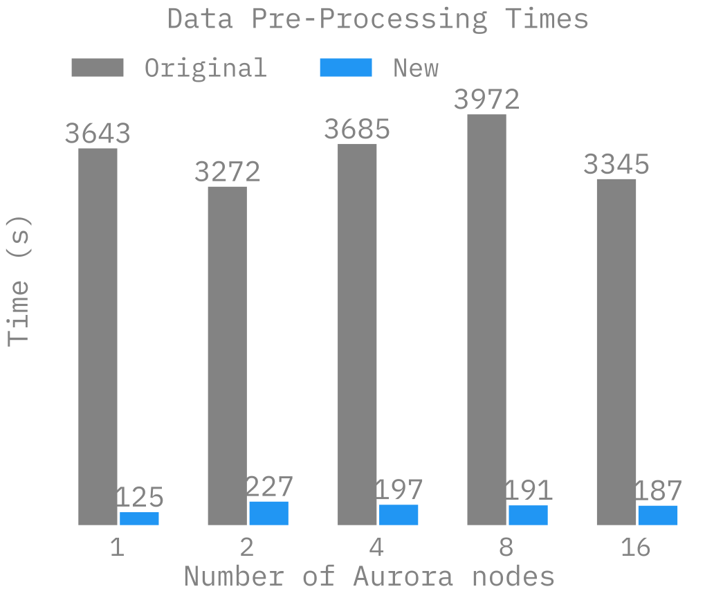
Concatenation forgets: order becomes a hyperparameter
Domain weights honored per batch, deterministically
BlendCorpus: aggregate → sample → index

Time to prepare 2T tokens: serial ~1 hr vs distributed ~2 min, a 30x speedup — Index-build time for 2T tokens: serial ~1 hr vs distributed ~2 min (**30x**).

Reproducibility and the fork tax

Same seed + shards + weights → same batch, every rank, every run.

Universal:

data churn: re-scraped shards break determinism
pin everything: SHAs · tokenizer · shard lists · weights

If you fork upstream (we fork torchtitan for XPU):

upstream churn: 46 syncs in 7 weeks, any can shift RNG

Every fork sync runs a deterministic smoke test first:

flowchart TB A["start upstream @ HEAD"] --> B["resync · 50 steps · deterministic smoke test"] B --> D{"bit-exact?"} D -->|✅| C["diff = 0 ✓ ship"] D -->|❌️| F["diff ≠ 0 bisect + fix"] F -.->|retry| B classDef source fill:#7c4ed508,stroke:#7c4ed5,color:#7c4ed5,stroke-width:1.5px classDef stage fill:#118cc208,stroke:#118cc2,color:#118cc2,stroke-width:1.5px classDef ship fill:#1da81108,stroke:#1da811,color:#1da811,stroke-width:1.5px classDef gate fill:#ee8f2410,stroke:#ee8f24,color:#c9750f,stroke-width:1.5px classDef bad fill:#e0556008,stroke:#e05560,color:#e05560,stroke-width:1.5px class A source class B stage class D gate class C ship class F bad

Bit-exact = loss + grad-norm + peak memory match baseline.

Determinism is the whole game: same seed + same shards + same blend weights must give the same batch on every rank, every run. Two things threaten it. Upstream churn: we live on a fork of TorchTitan and upstream moves fast (46 syncs in 7 weeks), any one of which can silently shift dataloader or RNG behavior. Data churn: corpora get re-scraped and re-shuffled, and if the shards move under you “reproducible” is a lie. So we pin everything: exact repo SHAs, tokenizer version, shard file lists, blend weights, all committed with the run.

The war story: an upstream commit that “just refactored the dataloader” changed shuffle order and quietly changed the loss curve. Bit-exact loss + grad-norm + peak-memory on 50 deterministic steps is cheap insurance. The “fork tax”: forking buys you XPU support, and the bill comes due as continuous upstream-sync work.

A Python environment that works

Don’t build from scratch. Layer on the site module: it already has torch, MPI, and the GPU stack built for this machine.

# 1. the site's prebuilt module (torch / MPI / GPU)
module load frameworks

# 2. a venv on top -- your packages, inheriting the module's torch
uv venv --system-site-packages --python python3 .venv
source .venv/bin/activate
uv pip install "git+https://github.com/saforem2/ezpz"   # resolves in seconds

The rule:

venv first, clone last

--system-site-packages is what lets the venv see the module’s torch (skip it and you pull a fresh CPU-only wheel)
never pip install into base; clone conda base only if a package hard-requires conda (slow, huge)

The most common way to lose your first hour on a supercomputer is a broken env. Start from the site’s prebuilt frameworks module (on Polaris that is module use /soft/modulefiles; module load conda; conda activate base), then back. Build the venv with --system-site-packages so it sees the module’s prebuilt torch instead of pulling a fresh CPU-only wheel. I use plain .venv here for clarity, but in practice name it after $CONDA_PREFIX (venvs/$(basename $CONDA_PREFIX)) so you get one venv per frameworks release and a module bump does not silently mix ABIs. One uv venv gotcha: it defaults to a uv-managed CPython download, which would build the venv against the wrong interpreter and inherit the wrong site-packages, so pin it to the module’s python with --python python3 (uv resolves it on PATH). Then uv pip install (not plain pip) resolves and installs in seconds, a real difference on a shared login node, and honors the --system-site-packages venv so it still picks up the module’s prebuilt torch. Clone base only if some package truly requires conda: cloning copies the entire env, it is slow and huge and gets out of hand fast. venv first, clone last.

Why `import` melts Lustre at scale

One import torch = thousands of stat() / open(). Now × 50,000 ranks.

Metadata server chokes, not bandwidth
Laptop-seconds → cluster-minutes before step 1
Per-file rsync past 256 nodes: 1-2 hours

Python is pathologically small-file

The fix is not a faster FS. It is not hitting the FS from every rank.

Deep dive: Running 50k Python processes on Aurora with ezpz yeet

A single import torch is not one file read: it is thousands of stat(), open(), and read() calls walking site-packages for modules, .pyc caches, and shared objects. Run that on 50,000 ranks at once, all pointed at the same shared filesystem, and the bottleneck is not bandwidth: Lustre has plenty of throughput, but the metadata server chokes on millions of tiny concurrent stat()s.

Every rank independently discovers the same tree; metadata ops serialize on a small number of servers; startup that takes seconds on your laptop takes minutes before the first training step, paid every job. A per-file rsync of an env to all nodes was projected at 1 to 2 hours past 256 nodes, because the per-file metadata cost dominates, not the data. The HPC intuition already applies: avoid small files. Python is pathologically small-file. The fix is not a faster filesystem, it is not hitting the shared filesystem from every rank, which sets up yeet next.

`ezpz yeet`: broadcast the environment

Copy the env once to node-local /tmp, fan out node-to-node. Imports hit local SSD.

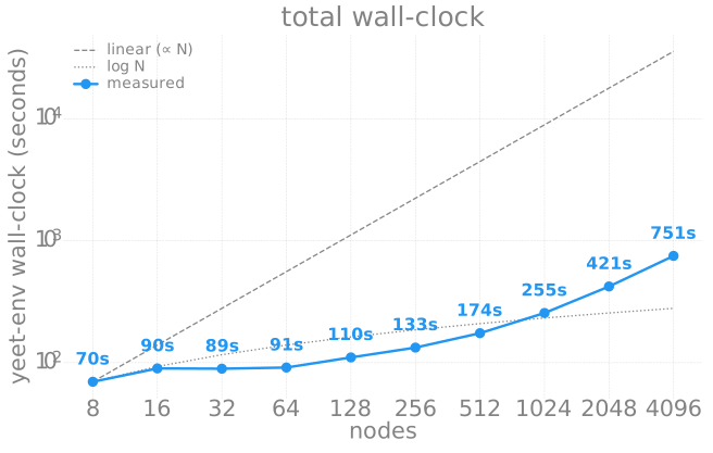
ezpz yeet --compress          # 1 tarball off Lustre
source /tmp/.venv/bin/activate
ezpz launch python3 -m your_app.train

Greedy O(log N) fan-out tree, not a star
Per-node cost 8.7s → 0.18s (48x)
Full Aurora: pre-launch under 13 min

Instead of 50k ranks each clawing at Lustre, copy the env once to node-local /tmp and fan it out node-to-node; imports then hit local SSD. Modes: --compress (tar.gz, copy one file, extract locally, least metadata I/O), --copy (cp -a for a fast initial copy), and the default rsync (only sends diffs after a pip install). After yeet, activate /tmp/.venv and cd back to your project so data/outputs stay on the shared FS.

Measured 8 to 4096 nodes on Aurora, two regimes: 8-64 nodes extract-bound (~70-91s flat), ≥128 broadcast-bound (each 2x adds ~1.5-1.8x). The one-tarball trick is why it scales: it turns the Lustre side into a single sequential read regardless of node count, so only the broadcast scales with N. The old per-file rsync mode was the 1-2 hour disaster from the previous slide. The next slide shows why it stays O(log N): the greedy fan-out tree.

Why it stays `O(log N)`: greedy fan-out

A single source saturates its NIC at ~8 outbound copies. So each node that finishes becomes a source for the next batch: the tree grows recursively.

flowchart LR S(["source (shared FS)"]) --> L["node00 /tmp"] L --> A1["node01"] L --> A2["node02"] L --> Ad["…"] L --> A8["node08"] A1 --> B1["node09"] A1 --> Bd["…"] A1 --> B8["node16"] A2 --> C1["node17"] A2 --> Cd["…"] A2 --> C8["node24"] classDef src fill:#ee8f2410,stroke:#ee8f24,color:#ee8f24,stroke-width:1.5px classDef g1 fill:#118cc210,stroke:#118cc2,color:#118cc2,stroke-width:1.5px classDef g2 fill:#1da81110,stroke:#1da811,color:#1da811,stroke-width:1.5px classDef dots fill:#83838308,stroke:#83838388,color:#838383,stroke-width:1px class S,L src class A1,A2,A8 g1 class B1,B8,C1,C8 g2 class Ad,Bd,Cd dots

Cap 8 outbound / source; a thread pool load-balances to the least-busy one
Faster nodes don’t wait: finish early → serve early
Result: ~O(log N) wall-clock, not the O(N) of a single-source star

This is the mechanism behind the O(log N) curve on the previous slide, straight from the yeet write-up. A single source can only push to about 8 nodes before its NIC saturates, so yeet uses a greedy streaming fan-out: a single thread pool manages all rsyncs, each source capped at MAX_PER_SOURCE=8 concurrent outbound transfers. As each rsync completes, that node is registered as a new source, and new transfers go to whichever source has the fewest active ones (load-balanced). The tree grows recursively: source to node00, node00 to gen-1 (node01..08), each of those to gen-2, and so on. Faster nodes don’t wait for slower ones: if node01 finishes in 15s but node08 takes 30s, node01 is already serving new targets. That is why the wall-clock is approximately O(log N) at moderate scale rather than the O(N) you’d get pushing from one source.

Bethany covered these in depth. Fast recap as a decision menu: five axes, mix and match (“4D parallelism” = several stacked). The only question: what each splits.

Strategy	Abbr.	What it splits	You reach for it when…
Data Parallel	`DP`	the batch: every GPU holds a full model copy, sees different data	the model fits on one GPU
Tensor Parallel	`TP`	individual weight matrices across GPUs (within a layer)	a single layer is too big; needs fast interconnect
Pipeline Parallel	`PP`	the model by layer (stages), streaming micro-batches through	the model is deep and will not fit vertically
Sequence / Context	`SP`	the sequence dimension (long context) across GPUs	context length blows up activation memory
Expert Parallel	`EP`	experts of an MoE layer across GPUs	you are training a Mixture-of-Experts

Read it as a hierarchy of cost

DP is nearly free (no model changes). TP is chatty (all-reduce inside every layer, keep it on-node). PP needs careful micro-batch scheduling. Add them in that order of pain.

In pictures (1/2): replicate, shard, split a layer

Data Parallel — model replicated, batch sliced, grads averaged

flowchart LR x0["x0"] --> N0["NN → Loss"] x1["x1"] --> N1["NN → Loss"] N0 --> A["avg grads"] N1 --> A classDef d fill:#f2b8b508,stroke:#e05560,color:#e05560,stroke-width:1.5px classDef m fill:#f9d79508,stroke:#ee8f24,color:#c9750f,stroke-width:1.5px classDef g fill:#83838310,stroke:#838383,color:#838383,stroke-width:1.5px class x0,x1 d class N0,N1 m class A g

FSDP / ZeRO — params sharded, all-gathered just-in-time per layer

flowchart LR G0["GPU0 shard A"] <-->|"all-gather"| G1["GPU1 shard B"] G1 <-->|"all-gather"| G2["GPU2 shard C"] classDef s fill:#f9d79508,stroke:#ee8f24,color:#c9750f,stroke-width:1.5px class G0,G1,G2 s

Tensor Parallel — each layer’s matmul sliced; all-reduce every layer

flowchart LR subgraph GPU0 A0["Layer k · half A"] end subgraph GPU1 A1["Layer k · half B"] end A0 <-->|"all-reduce (every layer)"| A1 classDef t fill:#118cc208,stroke:#118cc2,color:#118cc2,stroke-width:1.5px class A0,A1 t

DP is the default (nothing changes). FSDP trades comms for memory. TP is chatty (all-reduce every layer): keep it on-node.

The five strategies from the table, now as pictures (the cartoon from our pretraining paper, redrawn), split over two slides. This first slide is the three that either replicate or shard the model itself. Data parallel: the model is replicated on every GPU, the batch is sliced (x0/x1/…), and gradients are all-reduced and averaged each step; it is the default and costs almost nothing. FSDP/ZeRO: parameters, gradients, and optimizer state are sharded across GPUs and all-gathered just-in-time as each layer runs forward, trading communication for memory. Tensor parallel: each layer’s matmul is split across GPUs with an all-reduce of activations every single layer, so it is chatty, keep it on-node where the interconnect is fast. Next slide: the two that split along the compute / sequence axis (pipeline and sequence/context).

In pictures (2/2): split the depth, split the sequence

Pipeline Parallel — layer stack split into stages; micro-batches pipelined

flowchart LR subgraph GPU0 direction LR L0["L0"] --> L1["L1"] end subgraph GPU1 direction LR L2["L2"] --> L3["L3"] end L1 -->|"stage hand-off"| L2 classDef p fill:#1da81108,stroke:#1da811,color:#1da811,stroke-width:1.5px class L0,L1,L2,L3 p

Sequence / Context — sequence sliced per rank; ring-attention rotates KV

PP splits the layer stack into stages across nodes; SP/CP splits the sequence for long context (ring-attention over KV). EP (not shown) splits MoE experts.

ZeRO / FSDP: the memory vs comms trade

Still data parallel: shard the replicated state, gather on demand. Each stage shards one more thing, so per-GPU memory drops.¹

ZeRO / FSDP memory partitioning: horizontal memory-proportional bars per GPU across four stages (Baseline/DDP, ZeRO-1 shard optimizer, ZeRO-2 +gradients, ZeRO-3/FULL_SHARD shard everything). Each stage replaces a full-width component bar with a 1/N per-GPU slice over a greyed freed-memory track, so per-GPU memory drops from 16 GB toward 16/N GB. — Each stage shards one more component into a 1/N per-GPU slice; the greyed track is memory freed on that GPU.

The trade

Buy memory with comms: an all-gather per step. More stages = less memory, more comms.

✅ model almost fits, or you want a bigger batch
❌ a single layer won’t fit → that’s TP / PP

Plain data parallelism replicates everything on every GPU: params, gradients, optimizer states. For an Adam-trained model that is the same tensor stored dozens of times over. ZeRO (DeepSpeed) and FSDP (PyTorch) shard those replicated tensors across the DP group and gather each piece back only when a GPU needs it. Stage 1 shards optimizer states (the biggest first win: Adam states are ~2x the params), stage 2 adds gradients, stage 3 adds params (that is FSDP’s default full shard).

The trade: you buy memory with communication, an all-gather to reconstruct the shard each forward/backward, then a re-shard. Worth it when the model almost fits or you want a bigger batch: you stay in a pure-DP mental model, no model surgery, and pay a comms tax instead of buying more GPUs. Not worth it when a single layer does not fit: sharding a replica will not save you, that is a TP/PP problem. The framing for the room: ZeRO/FSDP is still data parallelism, you just change how the DP group stores state, which is why it is the first thing to try when you are memory-bound but the architecture still fits layer-wise.

What you’ll actually pick

Climb only when memory forces you: DP → FSDP/ZeRO → TP → PP.

Fits on one GPU → DP, scale batch
Almost fits → FSDP/ZeRO (stage 1, then 3)
A layer won’t fit → TP on-node, PP across
Long context → SP · MoE → EP

Tip

ezpz launch Same script, every machine. No mpiexec / srun / bind wrappers.

%%{init: {'themeVariables': {'fontSize': '22px'}, 'flowchart': {'nodeSpacing': 55, 'rankSpacing': 45, 'padding': 14}}}%% flowchart LR EZ(["ezpz launch"]) EZ --> AURORA["PBS · Intel Aurora"] EZ --> POLARIS["PBS · NVIDIA Polaris"] EZ --> PM["SLURM · NVIDIA Perlmutter"] EZ --> FRONTIER["SLURM · AMD Frontier"] EZ --> MAC["Multi-CPU"] classDef hub fill:#ee8f2408,stroke:#ee8f24,color:#ee8f24,stroke-width:1.5px classDef aurora fill:#3b82f608,stroke:#3b82f6,color:#3b82f6,stroke-width:1.5px classDef polaris fill:#10b98108,stroke:#10b981,color:#10b981,stroke-width:1.5px classDef perlmutter fill:#06b6d408,stroke:#06b6d4,color:#06b6d4,stroke-width:1.5px classDef frontier fill:#ef444408,stroke:#ef4444,color:#ef4444,stroke-width:1.5px classDef mac fill:#a78bfa08,stroke:#a78bfa,color:#a78bfa,stroke-width:1.5px class EZ hub class AURORA aurora class POLARIS polaris class PM perlmutter class FRONTIER frontier class MAC mac

Before you commit: find the learning rate

The last knob before a full-machine run. Sweep the LR on a short run and read the curve, don’t guess a number and burn 2k nodes finding out it was wrong.

flat/high at small LR: trains, just slowly
basin: loss drops into the usable band
cliff: one step too big → grads to inf → NaN
pick just below the cliff: the fastest rate that still has safety margin as the run heats up

Cheap insurance

A few hundred steps to sweep saves a full-scale run that NaNs at step 7.

Conceptual LR-finder: loss vs learning rate on a log axis, flat at small LR, a basin (sweet spot, circled) in the middle, then a steep cliff diverging to NaN at large LR

The last thing to settle before you spend real machine time. An LR-finder is a short run where you ramp the learning rate across a log-spaced sweep and watch the loss. Three regions: at small LR the loss is flat and high because each step barely moves the weights; there is a basin where it actually trains; and past a cliff the step is too large, the gradient norm blows to inf one step before the loss, and you NaN. Pick a rate just below the cliff, not exactly at the minimum, because the minimum has no headroom once the run warms up, the batch grows, or numerics drift. Do this cheaply at small scale: a few hundred steps of sweep is nothing against a 2k-node run that dies at step 7. This is the setup for the Part 2 story, where at 80B every optimizer we tried cliffed to NaN in the first dozen steps.

You’ve launched. Now everything tries to kill it.

Part 1 spent the compute well. Part 2 is about not wasting what you’ve spent.

See you after the break.

Part 2: now keep it alive

Part 1 got a run started. That was the easy part.

Not a program you start: one you babysit for weeks
Every crash you don’t recover is compute you already paid for, thrown away
So the question becomes: how cheaply do you recover when (not if) it breaks?

The rest of this talk

Good news: the loss curve. Bad news: everything that can interrupt it.

Where we’re headed: AuroraGPT-2B to 7.77T tokens

One continuous run, 154K steps, three data-mix stages. Everything in Part 2 is what it takes to keep this curve going.

AuroraGPT-2B loss vs tokens over one continuous 7.77T-token run: train and val loss track together, plateau, then step down sharply at each of two data-mix stage transitions (4.673T and 7.064T tokens), ending at loss 2.03. — Each data-mix transition (dashed) steps the loss down; train and val stay locked together to a final 2.03.

And the full picture: every run, one axis

Every canonical AuroraGPT pretraining run, loss vs tokens. Bigger models fall faster per token; the 2B reference rides three data-mix stages the furthest.

Training loss vs tokens for five overlaid AuroraGPT chains: 2B-MDS reference (blue dashed) descending through two data-mix stage transitions to 2.03 at 7.77T tokens; 2B torchtitan n256 (salmon) and n512 (dark red) tracking near 2.65-2.71; and the two 20B chains (n256 orange dashed, n512 green) dropping steeply per token to about 2.44. — The 20B chains (green, orange) drop fastest per token; the 2B-MDS reference (blue) goes furthest, stepping down at each data-mix transition to 2.03.

Batch size: the ceiling, and the knobs

$B_{\text{crit}}$ : the largest batch where more data-parallel workers still buy near-linear speedup.²

Speedup vs global batch on log-log axes. An actual (blue) speedup curve tracks the ideal linear reference closely at small batch (green 'near-linear' region, labelled '2x batch is about half the steps'), then bends away and flattens past a red dashed B_crit marker (grey 'speedup saturates' region).

The ceiling

below: 2x batch ≈ half the steps, more nodes nearly free
above: speedup saturates, training gets unstable³⁴
HPC hits it first: INCITE jobs want ~2k nodes, past $B_{\text{crit}}$
fix is TP/PP/EP + a batch you chose, not “more DP”

The knobs (and where they break)

LR scaling (linear / $\sqrt{B}$ )² + longer warmup + grad clip
linear LR backfires: 80B NaN’d earlier (step 7 vs 29)
LRs don’t transfer: mano@48 loses to AdamW@384 (unless you use μP⁵)

Tip

Scheduling (grab the machine) and the math (stay under $B_{\text{crit}}$ ) pull opposite ways. Re-tune at the target batch and node count, don’t extrapolate a small-batch LR up a 100x jump and hope.

The critical batch size is the largest batch where adding data-parallel workers still buys near-linear speedup. Below it, doubling the global batch roughly halves the steps to a target loss, so more nodes means less wall-clock, nearly free. Above it, speedup saturates: you burn more tokens and compute for the same loss, sample efficiency drops, and training gets unstable.

Why HPC folks hit this wall first: INCITE-scale jobs want at least 20% of the machine, about 2k nodes on Aurora. Pure data-parallel at that node count means a very large global batch, straight past B_crit. The fix is not “more DP”, it is TP/PP/EP plus a batch you actually chose. B_crit grows with model and data scale but sub-linearly, so it is a moving target you measure, not assume.

The knobs for actually running a large batch: raise the LR with the batch (linear or sqrt-B) so each step still moves the weights meaningfully; use longer warmup as the batch grows to survive the noisy early steps; and lean on stability aids like grad clipping, a large-batch-tuned optimizer such as LAMB, and a decent epsilon. Where they break: past B_crit sample efficiency degrades. Linear LR scaling backfires at the extreme; at 80B, LR-scaling the 16x batch moved the NaN earlier, step 7 vs step 29. And LRs do not transfer across batch: mano tuned at GBS=48 loses to AdamW at GBS=384 (2.88 vs 2.71) until re-tuned. Practical rule: re-tune at the target batch and node count, or sidestep the re-tuning entirely with muP (maximal- update parametrization): parametrize so the optimal LR is width-invariant, tune on a small proxy model, and transfer the hyperparameters to the full-scale run.

`mano`: Muon quality at AdamW speed

mano⁶ normalizes updates on a rotating Oblique manifold with $O(\text{dim})$ vector-norm ops (no Newton-Schulz iterations). So it matches Muon’s loss without Muon’s throughput tax.

Optimizer	Loss	TPS
Muon	3.557	4,556
`mano`	3.631	7,048
AdamW	3.801	7,245
SophiaG	4.719	7,208

Muon and mano tie on loss (~3.6); mano runs at AdamW speed (~7,000 vs ~4,600 TPS), so it wins on wall-clock.
Caveat: at large batch (GBS=384) AdamW still wins (2.71 vs 2.88); mano’s LR was tuned at GBS=48 and needs re-tuning.

Training loss vs step for Muon, mano, AdamW, SophiaG at 2B / GBS=48 over 1000 steps: mano and Muon converge lowest and nearly overlap, AdamW above, SophiaG highest

Second-order optimizers: the landscape

AdamW is the baseline. Everything else buys curvature at some compute price.

Optimizer	Core idea
AdamW⁷	diagonal 2nd moment + decoupled weight decay
SophiaG⁸	clipped Hessian-diagonal: light curvature, cheap
Shampoo⁹	Kronecker-factored preconditioner per layer
SOAP¹⁰	Adam in Shampoo’s eigenbasis: stabler, fewer knobs
Muon¹¹	Newton-Schulz orthogonalize: a cheap Shampoo-like step

Shampoo → SOAP → Muon is one family: same second-moment structure, cheaper each step. SophiaG takes the other cheap route: a clipped diagonal Hessian.¹²

AuroraGPT-2B optimizer comparison at 50M tokens/batch on 256 nodes. Left: training loss (log) vs consumed tokens for AdamW, Lamb, Muon, SophiaG; SophiaG reaches the lowest loss. Right: gradient norm (log); Muon's grad norm spikes ~six orders of magnitude at ~1.1T tokens (divergence) while SophiaG stays lowest and bounded. — Real 2B runs at GBS 6,144: **SophiaG** reaches the lowest loss with bounded grad norm; **Muon** diverges at ~1.1T tokens.

AdamW is the baseline; everything else buys curvature, a better preconditioner, at some compute price. I keep the on-slide table to the four that carry the story: AdamW, then the Shampoo/SOAP/Muon family. Three others live in the footnote: LAMB (Adam plus a layer-wise trust ratio on the LR, unlocks huge batches), Adopt (drops the current grad from the second moment so it converges for any beta_2), and Sophia (a cheap clipped Hessian-diagonal preconditioner, light curvature).

Zoom in on the family since it is the cleanest to explain. Shampoo is preconditioned gradient descent: for each weight matrix it keeps a Kronecker-factored second-moment estimate (left factor from GG^T, right factor from G^T G) and steps along the preconditioned gradient. Powerful, but the eigendecompositions and extra knobs (grafting, epsilon, preconditioning power and frequency) make it expensive and fiddly at scale. SOAP’s trick: Shampoo’s preconditioner defines a rotated coordinate frame, its eigenbasis, so run plain Adam inside that frame and refresh the basis only every k steps because it drifts slowly, which amortizes the costly eigendecomposition. The paper’s hook is that 1/2-power Shampoo equals Adafactor-in-the-eigenbasis, so SOAP is the natural generalization: full Adam in that basis. Result is fewer hyperparameters (essentially AdamW plus the refresh frequency), more stability, the preconditioning win at close to Adam’s per-step cost. Their reported numbers are roughly 40% fewer steps and 35% less wall-clock vs AdamW, but those are the authors’ runs so I keep them off the slide. Muon is the cheaper cousin: it approximates the same spectral update with Newton-Schulz orthogonalization instead of an explicit eigendecomposition, skipping the basis machinery entirely. mano, next, chases the same quality-per-flop from the opposite direction: manifold normalization instead of eigenbases.

80B: one bf16 cliff, three dead optimizers

At 80B (dim=9216), every constant-finder LR NaN-ed in the first ~dozen steps: grad_norm went to inf one step before the loss, while loss was still flat (~12.9).

Optimizer	Died at	Signature
`mano`	step 5	grad NaN (diverged first)
AdamW	step 9	grad NaN
SophiaG	step 14	Hessian-term overflow, ~6,100 node-h

mano died first (step 5), despite the safest-looking LR band
shared failure across 3 → a bf16-at-dim=9216 corner, not tuning
fix: long warmup + grad clip; stable at TP=4 · LBS=1

80B LR-finder at GBS=6144: mano, SophiaG, AdamW, muon loss-vs-LR. AdamW and muon cliff straight to NaN with no minimum; mano and SophiaG reach a real U-minimum first — 80B LR-finder (GBS=6,144): **AdamW and muon cliff straight to NaN**; `mano` and SophiaG reach a minimum first, then blow up past it.

At 80B (dim=9216), every constant-LR finder NaN’d in the first dozen steps: grad_norm went to inf one step before the loss, while the loss was still flat around 12.9. The table: mano died at step 5, AdamW at step 9, SophiaG at step 14 (a Hessian-term overflow that burned about 6,100 node-hours before it went).

The lesson: mano, our 2B speed win, died first despite sitting in the safest-looking LR band, so early-step ranking does not predict sustained stability. And because all three failed, this is a corner-level instability, bf16 at dim=9216, not an optimizer-tuning problem; the grad-path triggers are LBS>1 and a large dp_degree. Fix in flight: long warmup (at least 200 steps) plus grad clipping, possibly an fp32 grad path. The stable corner today is TP=4, LBS=1, GBS=372, which ran 100/100 steps NaN-free (loss 12.93 down to 7.72) at about 9.8% MFU. The figure is the LR-finder at the production batch: AdamW and muon cliff straight to NaN with no usable minimum (x marks the diverged LRs), while mano and SophiaG reach a real minimum around 11.9 and 11.8 before SophiaG blows up.

At scale, failure is the default

You are running one job across thousands of nodes in lockstep. The job dies when any node dies, so cluster MTBF is roughly single-node MTBF divided by N.

one node fails ~once a year; put 16,000 in one job → ~44 failures/day

Run	Scale	Failures
Llama 3 405B¹³	16K H100s · 54 d	419 (1 every 3h); 99% auto-recovered
OPT-175B¹⁴	~1K A100s · 2 mo	35 manual restarts + 100+ hosts cycled
BLOOM-176B¹⁵	384 A100s · 3.5 mo	frequent loss spikes
GLM-130B¹⁶	768 A100s · 2 mo	spikes worsen; some NaN

Plan for the failure, not for the happy path.

You are running one job across thousands of nodes in lockstep. The job dies when any node dies, so cluster MTBF is roughly single-node MTBF divided by N. Say each node is healthy and fails on average once a year; put 16,000 of them in one job and that is about 44 failures a day, purely from expected value. The math is unforgiving and everyone who has done it confirms it.

Llama 3 405B: 16K H100s over 54 days saw 419 interruptions, about one every three hours, 99% auto-recovered. OPT-175B: roughly 1K A100s over two months needed 35 manual restarts and cycled 100-plus hosts. BLOOM-176B: 384 A100s over 3.5 months, frequent loss spikes handled with embedding-norm and checkpoint cadence. GLM-130B: 768 A100s over two months, spikes that got increasingly frequent, some recovered, some went NaN. The takeaway: plan for the failure, not the happy path.

The Lustre tax comes back, now on the write path

In Part 1 the shared-FS tax hit reads: staging the env off Lustre with ezpz yeet. Checkpointing hits the same wall from the other side.

reads (Part 1): every rank stat()s the same env → stage node-local
writes (now): every rank flushes a 232 GB checkpoint to the same MDS
same fix, same fan-out: coordinate the writes, don’t stampede

Why it’s worse for checkpoints

A stale env costs you a slow startup. A checkpoint write that contends with training collectives can take the whole job down (next slide).

Deliberate callback, not a re-teach. In Part 1 the shared-filesystem tax showed up on the read path: every rank stat()ing the same tens-of-thousands-of-files venv, which is why we stage node-local with ezpz yeet. The same wall is now in front of us from the other side, on the write path. When you checkpoint, every rank flushes its shard of a 232 GB checkpoint to the same metadata server and the same fabric.

The reason to re-raise it here rather than assume it: writes are more dangerous than reads. A slow env stage costs you minutes of startup. A checkpoint write that lands unbounded on the shared fabric contends with the training collectives and can stall or crash the whole job, which is exactly the async-checkpoint meltdown on the next slide. Same discipline as Part 1: coordinate and bound the fan-out instead of letting every rank hammer the MDS at once.

Checkpointing: what, when, how big

Your only insurance policy. Resume from the last one, everything since is wasted.

What goes in

model weights (fp32 master)
optimizer state (~2x the model)
LR sched, step, RNG, dataloader pos

How big (measured)

20B → 232 GB. Sync save stalls training ~23.6 s; reload is ~55-63 s (dominated by dcp.load).

When: the cadence tradeoff

too frequent: write overhead eats throughput
too rare: a crash throws away hours

EV rule: interval where wasted work on a crash ≈ write overhead. At a failure every few hours, and a ~24 s blocking save, that lands in the tens-of-minutes range.

The ~24 s stall is why you push it off the critical path → async, next.

A checkpoint is your only insurance policy: if the job dies you resume from the last one, so everything since then is wasted work. What goes in: model weights as the fp32 master, optimizer state (the big one, Adam-family is about 2x the model), and the LR scheduler, step count, RNG, dataloader position.

How big, measured on our runs and written up in the ezpz checkpoint-restart guide: the 20B checkpoint is 232 GB. A synchronous save blocks the training thread for about 23.6 seconds, and a reload runs about 55 to 63 seconds, dominated by the 232 GB dcp.load. For scale, restart time grows with the model: roughly 10 seconds for a debug model, 40 seconds at 2B (a 23 GB checkpoint), 60 seconds at 20B.

When: two costs pull against each other. Too frequent and the write overhead eats throughput; too rare and a crash throws away hours of compute. Expected-value rule of thumb: pick an interval where the expected wasted work on a crash, about half an interval times your failure rate, is comparable to the write overhead you are paying. With a 24-second blocking save and a failure every few hours, that lands in the tens-of-minutes range. The write cost is exactly why you want it off the critical path, which is asynchronous checkpointing.

Asynchronous checkpointing, and how it melted the cluster

Done right, async hides the 232 GB write behind the next few hundred steps: snapshot to host memory, flush on a background thread, bound the fan-out.

Per-save training-thread stall, sync vs async, at 2B (23 GB) and 20B (232 GB). Sync blocks on the full write (3.75s / 23.6s); async pays only a short stage + drain (1.05s / 5.4s), 3.6x and 4.4x less stall. — Sync blocks the training thread on the whole write; async pays only stage + drain while the GPUs keep going. Measured on Aurora (ezpz guide).

snapshot to host memory, then flush on a background thread
bound concurrency: cap ranks flushing at once
reload is ~55-63 s at 20B (dcp.load-bound)

The naive version took the job down

Unbounded async at 20B / 512N+ contends with training collectives on the same fabric. Bound the fan-out; write a .complete marker last.

Done right, async checkpointing hides the write behind compute. Snapshot to host memory on the training thread, which is fast, then hand off. A background thread stages then flushes the bytes to the filesystem while the GPUs keep training. And bound concurrency: cap how many ranks flush at once so you do not stampede the metadata server and the fabric simultaneously. The point is to overlap the 232 GB write with the next few hundred steps so cadence costs almost nothing.

The numbers, from the ezpz checkpoint-restart guide: at 20B the synchronous save blocks the training thread about 23.6 seconds. Async drops that to about 5.4 seconds, roughly a 1.7-second stage plus a 3.7-second drain of residual, so about 4.4x less stall, roughly 18 seconds handed back per save. (At 2B, a 23 GB checkpoint, it is 3.75 seconds sync versus about 1.05 seconds async, about 3.6x.) Mechanism: PyTorch Distributed Checkpoint, dcp.async_save with a fan-out start and a try-finalize-if-ready, and a .complete marker written last so incomplete checkpoints are skipped; finalize uses an MPI probe on MPI’s own communicator to avoid deadlocking with the xccl training group.

The naive version took the job down: at 20B/512N+, turning on async unbounded takes the whole job down because the 232 GB background write contends with training collectives on the same fabric and everything stalls. And the failure that hides inside checkpointing: a PBS mid-save kill once left a stale step-4500 placeholder directory; the sync path saw it, assumed the save was complete, and the run sat walltime-blocked for weeks. An —auto-retry relaunch finally drove it 4,400 to 5,400 cleanly. A half-written checkpoint is worse than no checkpoint, which is exactly why the bounded fan-out plus a .complete-marker-last discipline matters.

Restarting quickly

The recovery clock runs crash → first-step-back-training, not crash → “file exists.”

Reload fast (reload is ~55-63 s at 20B, dcp.load-bound)

stage node-local: ezpz yeet checkpoint-729 → /tmp, not 512 ranks pulling 232 GB off Lustre at once
same fan-out as the venv, any dir or tarball

Reload anywhere: converters

Megatron ⇄ 🤗 HF ⇄ ZeRO ⇄ Universal
Universal decouples from the parallelism layout → resume at a different TP/PP/DP than you saved at
the converted HF checkpoint is what you evaluate, serve, or fine-tune from

A checkpoint you cannot reload fast is only half an insurance policy. The recovery clock runs from crash to first-step-back-training, not from crash to “file exists.”

Reload fast: stage the checkpoint node-local. ezpz yeet ~/models/checkpoint-729 pushes it to /tmp on every node so the reload hits local SSD instead of every rank pulling 232 GB off Lustre at once. Reload itself is about 55 to 63 seconds at 20B, dominated by the dcp.load of that 232 GB. Same fan-out that stages the venv works on checkpoints and datasets, any directory or tarball.

Reload anywhere with checkpoint converters: Megatron, HF, ZeRO, Universal. The training-format checkpoint and the format you evaluate, serve, or fine-tune from are not the same thing. Universal decouples the checkpoint from the parallelism layout, so you can resume at a different TP/PP/DP config than you saved at, recovering on whatever the scheduler gives you, not only an identical allocation. And the converted HF checkpoint is the portable artifact everything after pre-training reads, so fast portable reload is not just a restart nicety, it is how the model leaves pre-training. (Post-training itself is Jane’s talk, not this one.)

”The restarts”: three layers of recovery

Bad-node failover, hang-watchdog, and PBS resubmit each operate at a different scope.

flowchart TB subgraph job["📋 JOB scope: PBS · hours"] JOB_TXT["crash / walltime → chained resubmit"] subgraph node["🖥 NODE scope: failover wrapper · minutes"] NODE_TXT["bad host detected → swap from spare pool"] subgraph proc["⏱ PROCESS scope: ezpz launch · seconds"] PROC_TXT["stdout idle ≥ N s → kill + backoff"] end end end classDef jobC fill:#118cc208,stroke:#118cc2,color:#118cc2,stroke-width:1.5px classDef nodeC fill:#ee8f2408,stroke:#ee8f24,color:#ee8f24,stroke-width:1.5px classDef procC fill:#1da81108,stroke:#1da811,color:#1da811,stroke-width:1.5px classDef jobTxt fill:transparent,stroke:none,color:#118cc2 classDef nodeTxt fill:transparent,stroke:none,color:#ee8f24 classDef procTxt fill:transparent,stroke:none,color:#1da811 class JOB_TXT jobTxt class NODE_TXT nodeTxt class PROC_TXT procTxt class job jobC class node nodeC class proc procC

flowchart TB subgraph proc["⏱ PROCESS · seconds"] PROC_TXT["stdout idle ≥ N s → kill + backoff"] end subgraph node["🖥 NODE · minutes"] NODE_TXT["bad host detected → swap from spare pool"] end subgraph job["📋 JOB · hours"] JOB_TXT["crash / walltime → chained resubmit"] end proc -- "process exit" --> node node -- "node exhaustion" --> job classDef jobC fill:#118cc208,stroke:#118cc2,color:#118cc2,stroke-width:1.5px classDef nodeC fill:#ee8f2408,stroke:#ee8f24,color:#ee8f24,stroke-width:1.5px classDef procC fill:#1da81108,stroke:#1da811,color:#1da811,stroke-width:1.5px classDef jobTxt fill:transparent,stroke:none,color:#118cc2 classDef nodeTxt fill:transparent,stroke:none,color:#ee8f24 classDef procTxt fill:transparent,stroke:none,color:#1da811 class JOB_TXT jobTxt class NODE_TXT nodeTxt class PROC_TXT procTxt class job jobC class node nodeC class proc procC

Inner loops catch most failures; outer loops catch the rest.

`--auto-retry`: bad-node failover, on tap

The NODE layer: allocate spares up front, swap them in on failure. Out of bash, into ezpz.

# 522 nodes allocated; train on 512, 10 auto-reserved as spare.
ezpz launch --auto-retry --nhosts 512 \
  -- python -m torchtitan.train …

bad-node → scrape host, swap spare, re-exec
config-bug guard: 2 attempts with zero step= → stop

Broke the 20B/512N stall: a stale placeholder → walltime-blocked weeks; relaunch drove it 4,400 → 5,400. Ships in ezpz#144.

flowchart TB START(( )) -->|"qsub / sbatch"| LAUNCH["ezpz launch --auto-retry"] LAUNCH -->|"run + idle watchdog exit 124 if 30 min silent"| CLASSIFY["classify exit parse trailer · crash patterns · SIGTERM"] CLASSIFY -->|"success rc = 0, no crash"| DONE["DONE rc = 0"] CLASSIFY -->|"walltime / stuck / no spares left"| STOP["STOP spares exhausted · stuck pre-training"] CLASSIFY -.->|"bad node (crash / hang) swap in spare, retry"| LAUNCH classDef launchC fill:#7c4ed508,stroke:#7c4ed5,color:#7c4ed5,stroke-width:1.5px classDef classifyC fill:#ee8f2408,stroke:#ee8f24,color:#ee8f24,stroke-width:1.5px classDef doneC fill:#1da81108,stroke:#1da811,color:#1da811,stroke-width:1.5px classDef stopC fill:#e0556008,stroke:#e05560,color:#e05560,stroke-width:1.5px classDef startC fill:#838383,stroke:#838383,color:#838383 class START startC class LAUNCH launchC class CLASSIFY classifyC class DONE doneC class STOP stopC linkStyle 4 stroke:#e05560,color:#e05560

The NODE layer of the cascade: allocate spares up front, swap them in on failure. This moved out of bash and into ezpz. Allocate 522, train on 512, keep 10 spare, and loop until success, walltime, or spare exhaustion.

It classifies each attempt’s exit as success, walltime, bad-node, or stuck-pre-training. On bad-node it scrapes the failing host from the log, swaps in a spare, and re-execs. It guards against config bugs: two consecutive attempts with zero step= markers and it stops, so you do not burn the whole spare pool on a broken run. It broke the 20B/512N stall: that stale step-4500 placeholder from a PBS mid-save kill had the sync chain walltime-blocked for weeks, and an auto-retry relaunch drove it 4,400 to 5,400 cleanly. Ships in saforem2/ezpz#144, same scraper as the bash-lib path with a pure-Python loop on top. The diagram is Fig. 5 from the paper: each inner run’s exit is reclassified, bad-node SIGTERMs trigger a spare-swap and retry (the dashed loop back to launch), while walltime, spare exhaustion, and stuck-startup are the terminal STOP outcomes the bash wrapper lacked.

The detector under it all: the idle-timeout watchdog

--auto-retry (previous slide) needs to know a job hung. A hang quiets stdout, so idle stdout is the signal, and this watchdog is what fires on it.

# --auto-retry turns the watchdog on for you (idle default = FAILOVER_IDLE_TIMEOUT).
# Standalone, without node failover: --timeout is the detector, --retries re-execs.
ezpz launch --timeout 600 --retries 3 \
    python -m torchtitan.train --config-file ./config.toml

--timeout SECONDS: kill if stdout goes idle (not walltime); exit 124
--retries N: bounded re-exec, backoff 5/10/20/40/60s. Mutually exclusive with --auto-retry (bounded per-process vs unbounded node-level)

stateDiagram-v2 direction LR [*] --> Running Running --> Hung: no stdout for N seconds Hung --> Killed: SIGTERM → SIGKILL Killed --> Running: backoff, re-exec

Fires on absence of progress, not a heartbeat ping (a hung job is “alive” by kill -0).

This is the primitive under the previous slide. —auto-retry can only swap a bad node once it knows the job is stuck, and this idle-stdout watchdog is how it knows. The problem: xccl on XPU silently ignores train_timeout_seconds, so a job stuck in a hung collective sits consuming the full PBS walltime instead of aborting. But every collective hang quiets stdout, since every rank blocks in the same call and nothing reaches the log. That silence is the signal.

—timeout SECONDS kills the launched process if its stdout goes idle, not walltime, for that many consecutive seconds, returning exit code 124 to match GNU timeout(1). Under —auto-retry the watchdog is on by default (matching FAILOVER_IDLE_TIMEOUT); pass —timeout 0 to disable it even there. —retries N is the standalone re-exec path: it re-executes on any non-zero exit, including the watchdog’s 124, up to N times, with backoff 5, 10, 20, 40, 60 seconds capped. It is mutually exclusive with —auto-retry, because —retries is bounded per-process retry and —auto-retry is unbounded node-level failover; you pick one. The watchdog fires on absence of progress, not a heartbeat ping; a hung job is alive by kill -0, which is exactly why a heartbeat can lie to you.

Scope caveat: it watches only the process ezpz launch spawns directly. If qsub runs a wrapper that internally invokes python train.py, the watchdog needs to live inside that script, or wrap the inner call with ezpz launch too.

It caught a real silent hang in production

Job 8505298, 2026-05-23. Trains steps 1-37, then the log goes silent. No traceback, no rank dying. Just dead.

Time (CT)	Event
21:06:41	step 37 logged · `loss 11.80 · tps 3,919`
21:36:41	30 min dead air · `ezpz launch --timeout=1800` SIGTERMs
21:36:43	wrapper classifies exit 124 to silent-hang (not walltime)
21:36:43	no traceback to scrape, so blind swap of rank-0 host
21:36:45	attempt 2 launches on swapped node set
21:57:49	walltime hit · step 296 · loss 5.68 · ckpts persisted

Three new pieces fired in sequence on a real hang: the --timeout=1800 watchdog, the exit 124 classification, and failover_swap_one_blind(). Unattended, 9:36 PM on a Friday. Full writeup.

None of this is theory. Job 8505298, 2026-05-23. Attempt 1 trains cleanly steps 1 to 37, then the log goes completely silent at step 37: no traceback, no MPI error, no rank dying, just dead. Walk the timeline: step 37 logged at 21:06, then 30 minutes of dead air until ezpz launch —timeout=1800 SIGTERMs at 21:36; the wrapper classifies exit 124 as silent-hang, not walltime; with no traceback to scrape it does a blind swap of the rank-0 host; attempt 2 launches on the swapped node set two seconds later and runs to walltime at step 296.

Three new pieces had to fire in sequence on a real hang to prove production-readiness: the —timeout=1800 watchdog, the exit 124 classification (distinct from PBS exit 143), and failover_swap_one_blind() for when no specific bad node can be identified. They did. The run kept going, unattended, at 9:36 PM on a Friday.

Where production stands

What the machinery above actually produced. The next few slides zoom in on these.

Run	Nodes	Steps	Tokens	Loss	Status
2B base	256	92,859	4.674T (100%)	2.65	✅ complete
2B-MDS ref	256	154,391	7.770T (166%)	2.03	✅ 3-stage reference
20B/512N	512	6,010	605B (13%)	2.44	advancing (auto-retry)
20B/256N	256	6,301	159B (3%)	2.44	advancing
80B	512	14	(NaN’d)	NaN	❌ optimizer cliff

Two 2B runs complete; both 20B chains advancing; the 80B hit the bf16 optimizer cliff (the wall from Part 2).

The flagship run: AuroraGPT-2B to 7.77T tokens

One continuous run, 154K steps, three data-mix stages. It rode the whole Part 2 machinery: async checkpoints, layered auto-restart, silent-hang recovery.

This is the flagship: AuroraGPT-2B, one continuous 154,000-step pretraining run to about 7.77T tokens, and the reason it is here rather than in the appendix is that it rode the entire Part 2 machinery, async checkpointing, the layered auto-restart cascade, the silent-hang watchdog, across weeks of wall-clock. The curve is the proof it survived: train (solid) and validation (dashed) loss stay locked together, which means no silent divergence, and each of the two data-mix stage transitions, at 4.673T and 7.064T tokens, steps the loss down cleanly, ending around 2.03. The x-axis is tokens, computed from the iteration count times the 50.3M tokens per step (GBS 6144 x seq 8192). Data pulled from the production W&B run. The next slides zoom out: every chain on one loss axis, then throughput/MFU, then the eval gate.

The whole program, one axis

Every canonical AuroraGPT pretraining run, loss vs tokens. Bigger models fall faster per token; the 2B reference rides three data-mix stages the furthest.

This is the zoom-out: every canonical production trajectory on one loss-vs-tokens axis, reproduced from the torchtitan combined-production chart. Five chains: the 2B-MDS SophiaG reference (blue dashed, the pre-torchtitan Megatron-DeepSpeed run, carried to 7.77T tokens, 166% of the 4.67T stage-1 target, ending at 2.03); the two 2B torchtitan v2 chains, n256 (salmon, to 4.67T / 100%) and n512 (dark red, to 3.07T / 66%); and the two 20B chains, n256 (orange dashed, a one-off to 158B) and n512 (green, the canonical 20B, to 605B). The reading: the 20B curves descend visibly faster per token than the 2B curves, which is the expected scaling signal, and the 2B-MDS reference goes furthest because it ran longest, stepping the loss down at each of its two data-mix transitions (dotted verticals at 4.67T and 7.06T). Every torchtitan chain here is stitched live from W&B across all its restarts via the repo’s canonical concat, so it reflects the current state of each run. The 20B-256 tokens use GBS 3072 (LBS=1), not the 6144 the shared registry assumes.

What it costs: throughput and MFU

Same chains, the compute side: sustained per-GPU throughput and how much of the hardware’s FLOPs we actually use.

Two panels vs tokens for the five chains. Left, tokens/sec/GPU: 2B-MDS sustains ~4,700, the 2B torchtitan chains ~2,500-3,200, the 20B chains ~350-450 (a 10x-bigger model does fewer tokens/sec/GPU). Right, model FLOPs utilization: the 20B chains run higher (~17-22%) than the 2B chains (~9-12%). — Bigger model = fewer tokens/sec/GPU but **higher MFU** (20B ~17-22% vs 2B ~9-12%): the 20B keeps the XPUs busier per step.

The compute-cost companion to the loss overlay: the same five chains, now on throughput and MFU, reproduced from panels 2 and 3 of the combined-production chart. Left panel, per-GPU tokens/sec: the 2B-MDS reference sustains about 4,700 tok/sec/GPU, the 2B torchtitan chains sit around 2,500 to 3,200 (n256 async a bit above n512 sync), and the two 20B chains are much lower at roughly 350 to 450, which is expected: a 10x-bigger model does far fewer tokens per second per GPU. Throughput is the per-GPU number torchtitan logs, not aggregated.

Right panel, MFU: this flips. The 20B chains run at roughly 17 to 22 percent model FLOPs utilization versus about 9 to 12 percent for the 2B, because the larger model has bigger matmuls that keep the XPUs busier per step, so even though its tokens/sec is lower, it is using the hardware more efficiently. MDS does not log MFU, so it is absent from the right panel (same as the source chart). Data: the 2B MDS throughput from its on-disk per-step CSV, the four torchtitan chains pulled live from W&B via the canonical concat, bin-meaned. The dips in the 2B-MDS throughput line are checkpoint/eval pauses, not slowdowns.

It learns: eval vs tokens, and the 20B is most efficient

Loss falling is necessary, not sufficient. The eval gate is what says the model learned, and per token the 20B pulls ahead of both 2B chains.

lm-eval accuracy vs tokens consumed on four benchmarks (HellaSwag, ARC-Easy, ARC-Challenge, Winogrande) for the 2B v2 256N and 512N chains, the 20B v2 512N chain, and the 2B-MDS reference. On every benchmark the 20B (green) rises far steeper per token, reaching ARC-Easy ~0.69 and HellaSwag ~0.63 by ~440B tokens, beating both 2B chains at matched token counts. — Four benchmarks vs tokens. The **20B (green) climbs steepest per token**: ARC-Easy ~0.69 by ~440B tokens, already past both 2B chains. More model per GPU-hour, made literal.

The payoff, and it ties straight back to the thesis. Loss going down is necessary but not sufficient; the lm-eval gate is what tells you the model actually learned. Four benchmarks (HellaSwag, ARC-Easy, ARC-Challenge, Winogrande), accuracy vs tokens consumed, for the two 2B torchtitan chains, the 20B 512N chain, and the 2B-MDS reference (the blue x, SophiaG).

The reading: on every benchmark the 20B (green) rises far steeper per token than either 2B chain. By about 440B tokens it is already at ARC-Easy ~0.69 and HellaSwag ~0.63, beating both 2B chains at matched token counts by a wide margin, roughly 8x more token-efficient. That is “the most model per GPU-hour” made literal: at a fixed token (compute) budget, the larger model gets you further. The 2B chains still climb nicely and plateau around 2T tokens (HellaSwag ~0.56, ARC-Easy ~0.65). Data from the committed eval tables in the ezpz docs. Post-training (CPT/SFT/GRPO) is Jane’s talk and out of scope here; this is pretraining eval only.

Putting it together: one resilient launch

Everything in Part 2 collapses into a startup ritual and a single launch line. Nothing here is aspirational: each flag is one we saw earn its keep.

# 1. stage the env node-local (off Lustre) · Part 1
ezpz yeet --compress
source /tmp/.venv/bin/activate

# 2. launch with all three recovery layers armed · Part 2
ezpz launch \
    --auto-retry \                 # NODE:    swap bad hosts from the spare pool
    --np 512 \                     #          (allocate 522, keep 10 spare)
    --timeout 1800 \               # PROCESS: kill on 30 min of stdout silence
    --retries 3 \                  #          re-exec with exponential backoff
    -- python3 -m torchtitan.train --config-file ./config.toml
# JOB layer: a chained PBS resubmit wraps the whole thing (hours scope)

Data blended + pinned, env broadcast off Lustre, checkpoints async and node-local-stageable, failures caught at process / node / job scope.
The person who launches this can close the laptop. The 9:36-PM-Friday silent hang recovered itself.

The whole talk in one line

It all serves one number: model quality per GPU-hour. Spend the compute well (Part 1), and make recovery so cheap that a failure wastes almost none of it (Part 2).

This is the payoff slide: everything in Part 2 collapses into a startup ritual and one launch line, and nothing here is aspirational, every flag is one we watched earn its keep. Walk the two blocks. First, stage the env node-local off Lustre with ezpz yeet and activate from /tmp, the Part 1 lesson. Then launch with all three recovery layers armed: —auto-retry is the NODE layer (allocate 522, train on 512, swap bad hosts from the 10 spare); —timeout 1800 plus —retries 3 is the PROCESS layer (kill on 30 minutes of stdout silence, re-exec with exponential backoff); and a chained PBS resubmit wraps the whole thing at the JOB layer, the hours scope.

The one-liner to land: at this scale you do not prevent failures, you make recovery so cheap that failure stops being an event. The person who launches this can close the laptop; the 9:36-PM-Friday silent hang from the previous slide recovered itself.

What generalizes, what doesn’t

Generalizes (vendor / site / model)

Bit-exact deterministic smoke gate after every upstream sync
lm-eval as ground truth for “is it actually learning?”
Spare-node failover wrapper: same idea on Slurm
Launcher / env autodetect: push vendor-shaped assumptions out of training code

Doesn’t (re-tune per config / hardware / version)

torch.compile decisions (helps dense, can hurt)
Collective tuning (CCL vs gloo fallbacks, NCCL/CCL env)
Optimizer stability at the bf16 corner: LR-finder rank ≠ sustained stability

The meta-lesson, and it maps onto the whole talk. What generalizes is the machinery, not the numbers: the deterministic smoke gate after every fork sync, lm-eval as the ground-truth “is it learning” signal, the spare-node failover wrapper (the same idea ports to Slurm), and launcher/env autodetect that keeps vendor-shaped assumptions out of training code. That is exactly the ezpz bet: make the portable thing portable.

What does not generalize, what you must re-tune for each config, hardware, and version: torch.compile decisions (it helps dense models but can hurt), collective tuning (CCL vs gloo fallbacks, the NCCL/CCL env soup), and above all optimizer stability at the bf16 corner, where the LR-finder’s ranking does not predict sustained stability (that is what killed the 80B). Know which bucket a given knob is in, so you spend your tuning time only on the things that actually need it.

What to take home

Five ways to get more model per GPU-hour:

The five lessons

Data prep is a distributed-systems problem. Tokenize once, blend by weight, pin everything for reproducibility.
Do not hit Lustre from every rank. Stage node-local; broadcast the env.
Add parallelism in order of pain: DP → FSDP/ZeRO → TP → PP, and stay under the critical batch size.
Loss is not ground truth. Gate on evals; a bit-exact smoke test catches silent corruption.
Do not prevent failures, recover cheaply. Async checkpoints + layered auto-restart.

Start here

🍋 ezpz (launch anywhere, --auto-retry, yeet): github.com/saforem2/ezpz · ezpz.cool
🧠 torchtitan fork (XPU + our experiments): github.com/saforem2/torchtitan
📚 blendcorpus (weighted data blending): github.com/zhenghh04/blendcorpus

Deeper write-ups

Try it yourself: FSDP + TP in four lines

Everything in this talk, runnable now. Copy-paste onto any of these machines.

# 1. bootstrap the ezpz environment (auto-detects the machine)
source <(curl -fsSL https://bit.ly/ezpz-utils) && ezpz_setup_env
uv pip install --no-cache --link-mode=copy "git+https://github.com/saforem2/ezpz"

# 2. smoke test first (always)
ezpz launch python3 -m ezpz.examples.test

# 3. full FSDP + TP pre-training
ezpz launch python3 -m ezpz.examples.fsdp_tp

Same script, every machine

No mpiexec / srun / bind wrappers: ezpz launch auto-detects the scheduler and device. Smoke-test before the real run, every time.

The hands-on close: everything in this talk is runnable right now, and the point of ezpz is that these exact four lines work unchanged on Aurora, Polaris, Perlmutter, Frontier, or a laptop. Step one bootstraps the environment: the ezpz-utils script auto-detects the machine and sets up the module + venv for you, then uv pip installs ezpz (no-cache and link-mode=copy so it works cleanly on the shared filesystem). Step two is the smoke test, ezpz.examples.test, which the whole talk says to run first every time, it is a couple of minutes and catches a broken env or a bad node before you burn an allocation. Step three is the real thing: ezpz.examples.fsdp_tp is a complete FSDP + tensor-parallel pretraining example, the parallelism from the cartoon slide in actual runnable code. ezpz launch handles the scheduler and device binding, so there is no mpiexec or srun to get wrong. Encourage people to grab a short interactive allocation and try it during the break.

samf.sh/talks/2026/08/03

Thanks

AuroraGPT team: Venkat Vishwanath, the AI/ML Group at ALCF, collaborators across ANL.

Argonne Leadership Computing Facility: Aurora time, Sunspot staging.

Intel: Intel Max 1550 XPU + oneAPI / XCCL / IPEX support throughout.

Code & docs

ezpz: github.com/saforem2/ezpz
torchtitan fork (experiments/ezpz): github.com/saforem2/torchtitan
These slides: samf.sh/talks/2026/08/03

This research used resources of the Argonne Leadership Computing Facility, which is a DOE Office of Science User Facility supported under Contract DE-AC02-06CH11357.

Questions?

Footnotes

Appendix: backup slides

Material that didn’t make the main path but is here for Q&A. Pull the full slides from the AuroraGPT-at-scale deck as needed:

Post-training: CPT · SFT · GRPO curves (covered in Jane’s talk)
MoE on Intel XPU: throughput and where it stands
AERIS: a production case study on the same stack
Failover engineering: the full silent-hang recovery write-up
Open questions we’d like this community’s help on

A field guide to what breaks

The cost is telling transient (retry, fine) from systemic (retry reproduces it).

Failure taxonomy grid: rows are where it broke (Hardware, Software, Network, System), columns are transient (retry and you're fine) vs systemic (retrying just reproduces it). Silent failures with no traceback (corrupt shard, bad upstream commit, collective hang) are marked as the dangerous ones.

Two axes matter. Where it broke, so you know who fixes it, and whether it is transient (retry and move on) or systemic (stop, or you corrupt the whole run).

By layer: hardware is ECC errors, dead XPU, thermal throttle, a bad node in your allocation. Software is CheckpointError from routing non-determinism, OOM, a bad upstream commit. Network is fabric flaps, gloo “Connection closed by peer”, collective hangs. System is Lustre stalls, PBS walltime, the scheduler handing you a node it should have drained.

Transient means one bad node, a flaked collective, a mid-save kill: retry on fresh hardware and you are fine. Systemic means a config bug, a corrupted shard, a silent numerical bug: retrying just reproduces it faster. The whole operational cost is telling these two apart. Retry a systemic fault and you burn the spare pool; halt on a transient one and you waste walltime you already paid for. The dangerous cells are the silent ones, marked with a dot: no traceback, the loss still looks fine. A bf16 master that freezes RMSNorm so lm-eval never moves, or a TP reduction that logs the loss one-twelfth too low: correct-looking curves, no crash, and only a bit-exact eval gate or smoke test catches them.

War story: the fabric that wouldn’t sit still

At full-machine scale the interconnect is never fully healthy. It shows up two ways:

Loud: gloo Connection closed by peer (job 8470102). You get an exit code.
Quiet: a collective just stops. Every rank blocks in the same all_reduce.

The quiet one is dangerous:

alive by kill -0, nothing crashed
xccl ignores train_timeout_seconds → eats full PBS walltime
job 8479579 hung at step 803, heartbeat still ticking

The one signal you can trust: a hang quiets stdout. Absence of progress is the detector (→ watchdog).

At full-machine scale the interconnect is never fully healthy. A link flaps, a switch hiccups, and one collective somewhere stops making progress. The loud version is gloo TCP “Connection closed by peer” a few hours in (job 8470102, 20B/256N); at least it crashed, so you get an exit code to act on. The quiet version is a collective that just stops: every rank blocks in the same all_reduce, waiting on a peer that will never answer.

The quiet version is the dangerous one. The process is alive by kill -0, nothing has crashed. On XPU, xccl silently ignores train_timeout_seconds, so the hung collective sits there consuming your entire PBS walltime. We watched job 8479579 (20B/512N) hang at step 803 with the heartbeat still ticking: alive, and doing nothing. The one signal you can trust is that a collective hang quiets stdout, because every rank is blocked in the same call so nothing reaches the log. Absence of progress is the detector, which is exactly what the watchdog keys on.

ZeRO: Memory Optimizations Toward Training Trillion Parameter Models (Rajbhandari et al. 2020), Fig. 7. Per-param Adam mixed-precision budget: 2 (fp16 params) + 2 (fp16 grads) + 12 (fp32 master + momentum + variance) = 16 bytes; sharding across N ranks drives the sharded piece toward 16/N. ↩
An Empirical Model of Large-Batch Training (McCandlish et al. 2018): LR and warmup both need to grow with batch, and the payoff flattens at the critical batch size. ↩ ↩²
How Does Critical Batch Size Scale in Pre-training? (Zhang et al. 2025). ↩
How to Set the Batch Size for Large-Scale Pre-training? (Zhou et al. 2025). ↩
μP (maximal-update parametrization): Tensor Programs V (Yang et al. 2022). Reparametrize so the optimal LR is invariant to width, tune on a small proxy, then transfer to the full model (“μTransfer”). ↩
mano: manifold-normalized optimization (2026). Implemented in our fork alongside SPAM (2501.06842). ↩
Decoupled Weight Decay Regularization (Loshchilov & Hutter 2019). ↩
Sophia: A Scalable Stochastic Second-order Optimizer (Liu et al. 2023). A clipped diagonal-Hessian preconditioner; SophiaG estimates the diagonal with the Gauss-Newton-Bartlett trick. ↩
Shampoo: Preconditioned Stochastic Tensor Optimization (Gupta et al. 2018). Kronecker factors of $GG^\top$ . ↩
SOAP: Improving and Stabilizing Shampoo using Adam (Vyas et al. 2024). Runs Adam in Shampoo’s eigenbasis, refreshed every $k$ steps. ↩
Muon: MomentUm Orthogonalized by Newton-Schulz (Jordan et al. 2024/2025). ↩
Also common: LAMB (You et al. 2020), layer-wise trust ratio for huge batches; Adopt (Taniguchi et al. 2024), converges for any $\beta_2$ ; Sophia (Liu et al. 2023), clipped Hessian-diagonal. ↩
Llama 3 herd of models (Meta AI, 2024), §3.3.2 (Training reliability). ↩
OPT-175B chronicles + dev log (Zhang et al., 2022). ↩
BLOOM: A 176B-Parameter Open-Access Multilingual Language Model (BigScience, 2022). ↩
GLM-130B: An Open Bilingual Pre-Trained Model (Zeng et al., ICLR 2023). ↩

samf.sh/talks/2026/08/03/ 1

Pre-Training LLMs on a Supercomputer

Roadmap

Who this is for

The stack

Data prep is the first wall

From raw corpus to tokens

Blending data, efficiently

Reproducibility and the fork tax

A Python environment that works

Why import melts Lustre at scale

ezpz yeet: broadcast the environment

Why it stays O(log N): greedy fan-out

The parallelism menu

In pictures (1/2): replicate, shard, split a layer

In pictures (2/2): split the depth, split the sequence

ZeRO / FSDP: the memory vs comms trade

What you’ll actually pick

Before you commit: find the learning rate

You’ve launched. Now everything tries to kill it.

Part 2: now keep it alive

Where we’re headed: AuroraGPT-2B to 7.77T tokens

And the full picture: every run, one axis

Batch size: the ceiling, and the knobs

mano: Muon quality at AdamW speed

Second-order optimizers: the landscape

80B: one bf16 cliff, three dead optimizers

At scale, failure is the default

The Lustre tax comes back, now on the write path

Checkpointing: what, when, how big

Asynchronous checkpointing, and how it melted the cluster

Restarting quickly

”The restarts”: three layers of recovery

--auto-retry: bad-node failover, on tap

The detector under it all: the idle-timeout watchdog

It caught a real silent hang in production

Where production stands

The flagship run: AuroraGPT-2B to 7.77T tokens

The whole program, one axis

What it costs: throughput and MFU

It learns: eval vs tokens, and the 20B is most efficient

Putting it together: one resilient launch

What generalizes, what doesn’t

What to take home

Try it yourself: FSDP + TP in four lines

Thanks

Footnotes

Appendix: backup slides

A field guide to what breaks

War story: the fabric that wouldn’t sit still

Footnotes

Why `import` melts Lustre at scale

`ezpz yeet`: broadcast the environment

Why it stays `O(log N)`: greedy fan-out

`mano`: Muon quality at AdamW speed

`--auto-retry`: bad-node failover, on tap